Log-normal and logistic-normal terminology

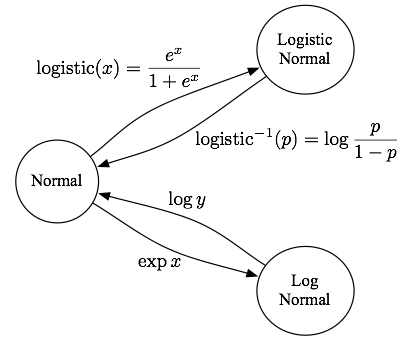
I was cleaning my office and found a back-of-envelope diagram Shay drew me once, so I’m writing it up to not forget.  The definitions of the logistic-normal and log-normal distributions are a little confusing with regard to their relationship to the normal distribution.  If you draw samples from one, the arrows below show the transformation to make it such you have samples from another.

For example, if x ~ Normal, then transforming as y=exp(x) implies y ~ LogNormal.  The adjective terminology is inverted: the logistic function goes from normal to logistic-normal, but the log function goes from log-normal to normal (other way!).  The log of the log-normal is normal, but it’s the logit of the logistic normal that’s normal.

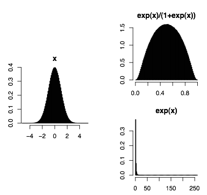
Here are densities of these different distributions via transformations from a standard normal.

In R:  x=rnorm(1e6); hist(x); hist(exp(x)/(1+exp(x)); hist(exp(x))

Just to make things more confusing, note the logistic-normal distribution is completely different than the logistic distribution.

What are these things?  There’s lots written online about log-normals.  Neat fact: it arises from lots of multiplicative effects (by the CLT, since additive effects imply the normal).  The very nice Clauset et al. (slides, blogpost) finds log-normals and stretched exponentials fit pretty well to many types of data that are often claimed to be power-law.

The logistic-normal is more obscure–it doesn’t even have a Wikipedia page, so see the original Aitchison and Shen.  Hm, on page 2 they talk about the log-normal, so they’re responsible for the very slight naming weirdness.  The logistic-normal is a useful Bayesian prior for multinomial distributions, since in the d-dimensional multivariate case it defines a probability distribution over the simplex (i.e. parameterizations of d-dim. multinomials), similar to the Dirichlet, but you can capture covariance effects and chain them together and other fun things, though inference can be trickier (typically via variational approximations).  A biased sample of text modeling examples include Blei and Lafferty, another B&L, Cohen and Smith, Eisenstein et al.

OK, so maybe these distributions aren’t really related beyond involving transformations of the normal.

Finally, note that the diagram only writes out the logistic-normal for the one-dimensional case; in the multivariate case, there’s an additional wrinkle that the logistic-normal has one less dimension than the normal, since you don’t need a parameter for the last one dimension (subtract the rest out of 1).  For example, a 3-d normal (distribution over 3-space) corresponds to a logistic-normal distribution over a simplex in 3-space, having only 2 dimensions.