AI and Social Science – Brendan O'Connor

Monte Carlo sampling algorithms (either MCMC or not) have a goal to attain samples from a distribution.  They can be organized by what inputs or prior knowledge about the distribution they require.  This ranges from a low amount of knowledge, as in slice sampling (just give it an unnormalized density function), to a high amount, as in Gibbs sampling (you have to decompose your distribution into individual conditionals).

Typical inputs include \(f(x)\), an unnormalized density or probability function for the target distribution, which returns a real number for a variable value.  \(g()\) and \(g(x)\) represent sample generation procedures (that output a variable value); some generators require an input, some do not.

Here are the required inputs for a few algorithms.  (For an overview, see e.g. Ch 29 of MacKay.)  There are many more out there of course.  I’m leaving off tuning parameters.

Black-box samplers: Slice sampling, Affine-invariant ensemble
- unnorm density \(f(x)\)

Metropolis (symmetric proposal)
- unnorm density/pmf \(f(x)\)
- proposal generator \(g(x)\)

Hastings (asymmetric proposal)
- unnorm density/pmf \(f(x)\)
- proposal generator \(g(x)\)
- proposal unnorm density/pmf \(q(x’; x)\)  .
… [For the proposal generator at state \(x\), probability it generates \(x'\)]

Importance sampling, rejection sampling
- unnorm density/pmf \(f(x)\)
- proposal generator \(g()\)
- proposal unnorm density/pmf \(q(x)\)

Independent Metropolis-Hastings: the proposal is always the same, but still have to worry about asymmetric corrections
- unnorm density/pmf \(f(x)\)
- proposal generator \(g()\)
- proposal unnorm density/pmf \(q(x’; x)\)

Hamiltonian Monte Carlo
- unnorm density \(f(x)\)
- unnorm density gradient \(gf(x)\)

Gibbs Sampling
- local conditional generators \(g_i(x_{-i})\)
… [which have to give samples from \( p(x_i | x_{-i}) \)]

Note importance/rejection sampling are stateless, but the MCMC algorithms are stateful.

I’m distinguishing a sampling procedure \(g\) from a density evaluation function \(f\) because having the latter doesn’t necessarily give you the former.  (For the one-dimension case, having an inverse CDF indeed gives you a a sampler, but multidimensional gets harder — part of why all these techniques were invented in the first place!)  Shay points out their relationship is analogous to 3-SAT: it’s easy to evaluate a full variable setting, but hard to generate them.  (Or specifically, think about a 3-SAT PMF \(p(x) = 1\{\text{\(x\) is boolean satisfiable}\}\) where only one \(x\) has non-zero probability; PMF evaluation is easy but the best known sampler is exponential time.)

And of course there’s a related organization of optimization algorithms.  Here’s a rough look at a few unconstrained optimizers:

Black-box optimizers: Grid search, Nelder-Mead, evolutionary, …
- objective \(f(x)\)

BFGS, CG
- objective \(f(x)\)
- gradient \(gf(x)\)

Newton-Raphson
- objective \(f(x)\)
- gradient \(gf(x)\)
- hessian \(hf(x)\)

Simulated annealing
- objective \(f(x)\)
- proposal generator \(g(x)\)

SGD
- one-example gradient \(gf_i(x)\)

I think it’s neat that Gibbs Sampling and SGD don’t always require you to implement a likelihood/objective function.  It’s nice to do to ensure you’re actually optimizing or exploring the posterior, but strictly speaking the algorithms don’t require it.

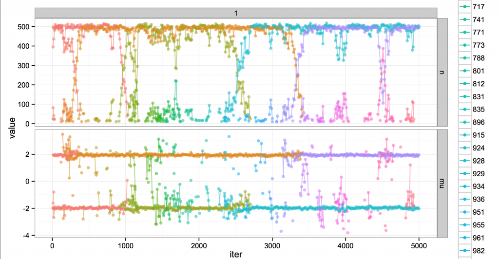
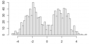
Here’s Gibbs sampling for a Dirichlet process 1-d mixture of Gaussians. On 1000 data points that look like this.

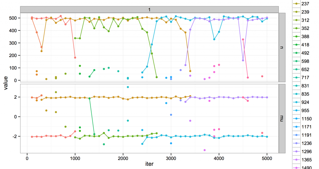
I gave it fixed variance and a concentration and over MCMC iterations, and it looks like this.

The top is the number of points in a cluster. The bottom are the cluster means. Every cluster has a unique color. During MCMC, clusters are created and destroyed. Every cluster has a unique color; when a cluster dies, its color is never reused.

I’m showing clusters every 100 iterations. If there is a single point, that cluster was at that iteration but not before or after. If there is a line, the cluster lived for at least 100 iterations. Some clusters live long, some live short, but all eventually die.

Usually the model likes to think there are about two clusters, occupying positions at the two modes in the data distribution. It also entertains the existence of several much more minor ones. Usually these are shortlived clusters that die away. But sometimes, they rise up and kick out one of the dominant clusters, and take over its space. This is evocative at least to me: for example, around iteration 2500 is a crisis of the two-mode regime, the fall of green and the rise of blue. (Maybe there are analogies to ideal points and coalitions or something, but call that future work…)

In fact the real story is a little more chaotic. Here’s the same run, but at finer resolution (every 10 iterations).

Around iteration 2500 you can see blue suddenly appear in green’s territory, where it’s bouncing around trying to get data points to convert to its cause. The clusters struggle and blue eventually wins out. Not all challenges are successful, though; e.g. at 1500 or 3600.

Ultimately, the dynamism is fake; looking at the broad sweep of history, it’s all part of a globally unchanging, static steady state of MCMC. The name of the cluster at mean -2 might change from time to time, but really, it occupies a position in the system analogous to the old regime.

Actually not just “analogous” but mathematically the same, as implied by CRP exchangeability; the cluster IDs are just an auxiliary variable for the DP. And the point of MCMC is to kill the dynamism by averaging over it for useful inference. This nicely illustrates you can’t directly use the actual clusters for averaging for an MCMC mixture model, since new clusters might slide into the place of old ones. (You might average over smaller spans, maybe; or perhaps look at statistics that are invariant to changing clusters, like the probability two datapoints belong to the same cluster. Or only use a single sample, which is at least guaranteed to be consistent?)

Technical details: this is actually a maybe-lame uncollapsed Gibbs sampler; I think it’s Algorithm 2 from Neal 2000 or something close. Everyone asks about the plots but they are easy to make; given a logfile with tuples like (iternum, cluster ID, n, mu), first melt() it, then ggplot with something like qplot(iternum, value, colour=factor(clusterID), data=x, geom=c(‘line’,'point’)) + facet_grid(~variable, scales=’free’).

Paul Moore posted a comment pointing out this great discussion of the correlation coefficient:

• Joseph Lee Rodgers and W. Alan Nicewander. “Thirteen Ways to Look at the Correlation Coefficient.” The American Statistician, Vol. 42, No. 1. (Feb., 1988), pp. 59-66. Link

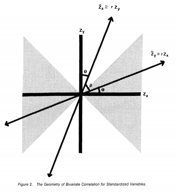
It’s related to the the post on cosine similarity, correlation and OLS. Anyway, I was just struck by the following diagram. It almost has a pop-art feel.

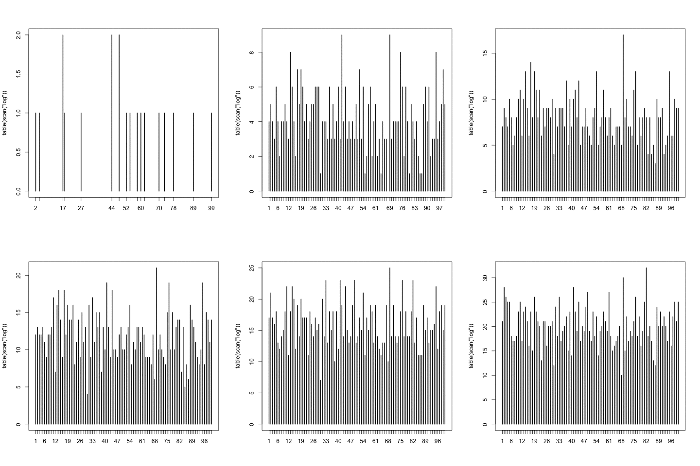
One of my favorite R tricks is scan(). I was using it to verify whether I wrote a sampler recently, which was supposed to output numbers uniformly between 1 and 100 into a logfile; this loads the logfile, counts the different outcomes, and plots.

plot(table(scan(“log”)))

As the logfile was growing, I kept replotting it and found it oddly compelling.

This was useful: in fact, an early version had an off-by-one bug, immediately obvious from the plot. And of course, chisq.test(table(scan(“log”))) does a null-hypothesis to check uniformity.

Really liking whoever made @SottedReviewer, e.g.

BEFORE I START TALKING ABOUT RANDOM FORESTS AND AUCS, I’LL THROW A BONE TO SOCIAL SCIENTISTS WITH A GRANOVETTER CITE. #ICWSM

— Sotted Reviewer (@SottedReviewer) March 11, 2013

There’s an entire great story here about ICWSM and interdisiplinariness or lack thereof. (Somehow I’ve never reviewed for ICSWM. Maybe I’m missing out.)

Larry Wasserman has a new position paper (forthcoming 2013) with a great comparison the Statistics and Machine Learning research cultures, “Rise of the Machines”. He has a very conciliatory view in terms of intellectual content, and a very pro-ML take on the research cultures. Central to his argument is that ML has recently adopted rigorous statistical concepts, and the fast-moving conference culture (and heavy publishing by its grad students) have helped with this and other good innovations. (I agree with a comment from Sinead that he’s going a little easy on ML, but it’s certainly worth a read.)

There’s now a little history of “Statistics vs Machine Learning” position papers that this can be compared to. A classic is Leo Breiman (2001), “Statistical Modeling: The Two Cultures”, which isn’t exactly about stats vs. ML, but is about the focus on modeling vs algorithms, and maybe about description vs. prediction.

It’s been a while since I’ve looked at it, but I’ve also enjoyed Jerome Friedman (1998)’s “Data Mining and Statistics: What’s the Connection?” which looks at what I’d now consider a kind of dark ages, the heuristic data mining approaches I associate with the 90′s.

I think Larry in 2013 would argue that NIPS or ICML-style mainstream ML research has substantially moved away from the crazy heuristic world of data mining and into something that looks more like statistical theory. Larry’s obviously focusing on areas he’s interested in. For example, current work in deep belief networks feels much more heuristicky — some of us (like me) think this area is very important and are sympathetic to the approach, though plenty aren’t — but of course the combination of theory and creative algorithmic innovation is useful to have even when they haven’t yet been reconciled. That’s what you get if you want to follow bleeding-edge research.

It’s always interesting to read this sort of thing. Before going to grad school I wrote a blog rant about stats and ML; it’s nice to actually know something about the topic now. Or conversely, maybe my worldview has been sufficiently shaped by all of Larry’s classes that I think the same way. Whatever.

A language model’s perplexity is exponentiated negative average log-likelihood,

$$\exp( -\frac{1}{N} \log(p(x)))$$

Where the inner term usually decomposes into a sum over individual items; for example, as \(\sum_i \log p(x_i | x_1..x_{i-1})\) or \(\sum_i \log p(x_i)\) depending on independence assumptions, where for language modeling word tokens are usually taken as the individual units. (In which case it is the geometric mean of per-token negative log-likelihoods.) It’s equivalent to exponentiated cross-entropy between the model and the empirical data distribution, since \(-1/N \sum_i^N \log p(x_i) = -\sum_k^K \hat{p}_k \log p_k = H(\hat{p};p)\) where \(N\) is the number of items and \(K\) is the number of discrete classes (e.g. word types for language modeling) and \(\hat{p}_k\) is the proportion of data having class \(k\).

A nice interpretation of any exponentiated entropy measure is as branching factor: entropy measures uncertainty in bits or nats, but in exponentiated form it’s measured as the size of an equally weighted distribution with equivalent uncertainty. That is, \(\exp(-H(p))\) is how many sides you need on a fair die to get the same uncertainty as the distribution \(p\).

Entropy differs by a constant depending whether you measured using base-2 or natural logarithms (then your units are bits vs. nats, respectively). But perplexity is the same with whichever base you want. The following works with base-2 instead:

\[ \exp(-\sum_k p_k \log p_k) = \exp(\sum_k \log p_k^{-p_k}) = \prod_k p_k^{-p_k} \]

Neat Wikipedia discovery: in ecology and economics, the diversity index measures were developed and they are in fact exponentiated entropy, just like perplexity. In fact, the different diversity indexes correspond to exponentiated Renyi entropies. The term “diversity” is a nice alternative term to “uncertainty” — less epistemologically loaded, just a description of the distribution.

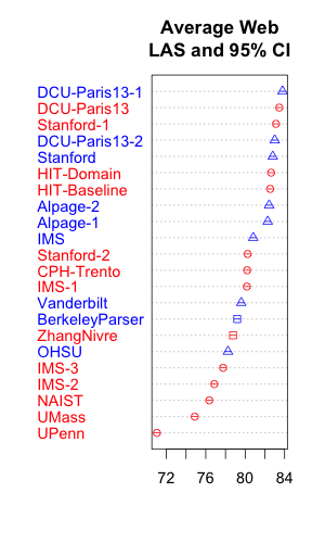
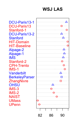
I was just looking at some papers from the SANCL-2012 workshop on web parsing from June this year, which are very interesting to those of us who wish we had good parsers for non-newspaper text. The shared task focus was on domain adaptation from a setting of lots of Wall Street Journal annotated data and very little in-domain training data. (Previous discussion here; see Ryan McDonald’s detailed comment.) Here are some graphs of the results (last page in the Petrov & McDonald overview).

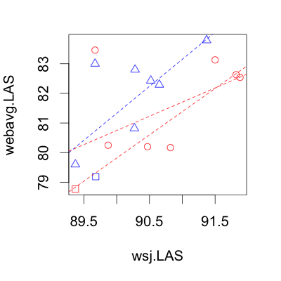
I was most interested in whether parsing accuracy on the WSJ correlates to accuracy on web text. Fortunately, it does. They evaluated all systems on four evaluation sets: (1) Text from a question/answer site, (2) newsgroups, (3) reviews, and (4) Wall Street Journal PTB. Here is a graph across system entries, with the x-axis being the labeled dependency parsing accuracy on WSJPTB, and the y-axis the average accuracy on the three web evaluation sets. Note the axis scales are different: web accuracies are much worse than WSJ.

There are two types of systems here: direct dependency parsers, and constituent parsers whose output is converted to dependencies then evaluated. There’s an interesting argument in the overview paper that the latter type seems to perform better out-of-domain, perhaps because they learn more about latent characteristics of English grammatical structure that transfer between domains. To check this, I grouped on this factor: blue triangles are constituents-then-convert parsers, and the red circles are direct dependency parsers. (Boxes are the two non-domain-adapted baselines.) The relationship between WSJ versus web accuracy can be checked with linear regression on the subgroups. The constituent parsers are higher up on the graph; so indeed, the constituent parsers have higher web accuracy relative to their WSJ accuracy compared to the direct dependency parsers. A difference in the slopes might also be interesting, but the difference between them is mostly driven by a single direct-dependency outlier (top left, “DCU-Paris13″); excluding that, the slopes are quite similar. Actually, this example probably shouldn’t count as a direct-dependency system, because it’s actually an ensemble including constituency conversion as a component (if it is “DCU-Paris13-Dep” here). In any case, lines with and without it are both shown.

Since the slopes are similar, we shouldn’t need varying-slopes hierarchical regression to analyze the differences, so just throw it all in to one regression (webacc ~ wsjacc + ConstitIndicator); so constituent parsers get an absolute 1.6% better out-of-domain accuracy compared to dependency parsers with the same WSJ parsing accuracy. (This is excluding DCU-Paris13.) It’s not clear if this is due to better grammar learning, or if it’s due to an issue with SD giving bad conversions on web text.

To see the individual systems’ names, here are both sets of numbers. These include all systems; for the scatterplot above I excluded the ones that performed worse than the non-domain-adapted baselines. (Looking at those papers, they seemed to be less elaborately engineering-heavy efforts; for example, the very interesting Pitler paper focuses on issues in how the representation handles conjunctions.)

CI’s can’t be seen on those skinny graphs, but they’re there; computed via binomial normal approximations using the number of tokens (i.e. assuming correctness is independent at the token level — though probably it should have sentence-level or doc-level grouping, of course, so they’re tighter than they should be.)

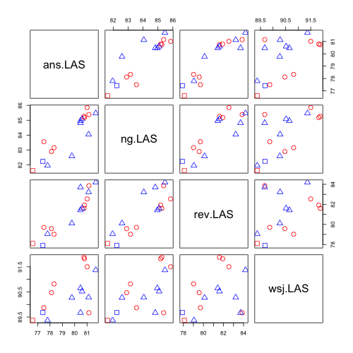
Finally, this is less useful, but here’s the scatterplot matrix of all four evaluation sets (excluding worse-than-baseline systems again).

All R code here.

There’s a lot to say about Powerset, the short-lived natural language search company (2005-2008) where I worked after college. AI overhype, flying too close to the sun, the psychology of tech journalism and venture capitalism, etc. A year or two ago I wrote the following bit about Powerset’s technology in response to a question on Quora. I’m posting a revised version here.

Question: What was Powerset’s core innovation in search? As far as I can tell, they licensed an NLP engine. They did not have a question answering system or any system for information extraction. How was Powerset’s search engine different than Google’s?

My answer: Powerset built a system vaguely like a question-answering system on top of Xerox PARC’s NLP engine. The output is better described as query-focused summarization rather than question answering; primarily, it matched semantic fragments of the user query against indexed semantic relations, with lots of keyword/ngram-matching fallback for when that didn’t work, and tried to highlight matching answers in the result snippets.

The Powerset system indexed semantic relations and entities (the latter often being wordnet/freebase nodes), did a similar analysis on the user query, then formed a database query against that index of semantic relations, synonym/hypernym expansions, and other textual information (e.g. word positions or gender identification). Then with all the rich (complicated) index information, you have neat features for ranking and snippet generation (i.e. query-focused summarization), but it’s so complicated it’s easy to screw up. (And don’t get me started on trying to run a segfault-prone Tcl/Prolog/C parser under an unstable 2006-era Hadoop…)

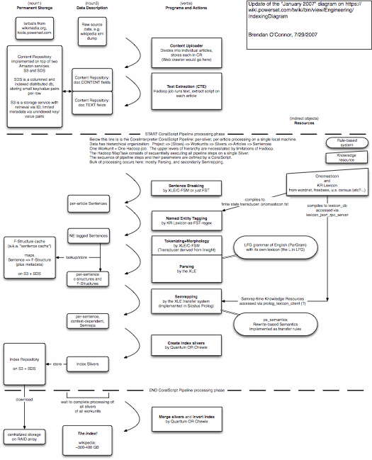
Here is a diagram I wrote in July 2007 to try to communicate internally what the entire system was doing. As you might imagine, it was difficult to keep everyone on the same page. This diagram only depicts the indexing pipeline; the query-time system would have required another diagram. NLP folks will note some rather surprising technology choices in some places. (Unweighted FST for NER? Yes. In fairness, it was eventually replaced by a statistical tagger. But the company did have >$12 million in funding at this point.)

As to whether this was “different than Google,” sure, I suppose. Certainly no serious search engine was crazy enough to do constituent parses (and unification parses, lexical lookups, coreference, etc.) of all sentences at index time — raising indexing costs, compared to keyword indexing, by perhaps 100x — but Powerset sure did.

It’s worth noting that since then, Google has added much more question-answering and structured information search, presumably using related but different techniques than Powerset used. (And Google even had some simple question-answering back then, as I recall; and, these days it’s said they parse the web all the time, at least for experimental purposes. They now have excellent groups of highly-regarded specialists in parsing, unsupervised lexical semantics, machine translation, etc., which Powerset never did.) And IBM’s Watson project more recently managed to produce a nice factoid question-answering system. In principle, deep semantic analysis of web text could be useful for search (and shallow NLP, like morphology and chunking, perhaps more so); but as the primary thing for a search startup to focus on, it seemed a little extreme.

As to what the “core innovation” was, that’s a loaded question. Was all this stuff useful? Usually I am cynical and say Powerset had no serious innovation for search. But that is just an opinion. Powerset developed some other things that were more user-visible, including a browser of the extracted semantic relations (“Factz” or “Powermouse”), a mostly separate freebase-specific query system (somewhat similar to Google’s recently released Knowledge Graph results), and completely separately, an open-source BigTable clone for index-time infrastructure (HBase, which has been developed quite a bit since then). In general, I found that design/UI engineering people respected Powerset for the frontends, scalability engineers respected Powerset for the HBase contributions, but NLP and IR experts were highly cynical about Powerset’s technology claims. If you get a chance, try asking researchers who were at ACL 2007 in Prague about Barney Pell’s keynote; I am told a number walked out while it was underway.

For good commentary on the situation at the time, see these Fernando Pereira blog posts from 2007: Powerset in PARC Deal, and Powerset in the NYT.

After the acquisition, Microsoft filed patent applications for all the Powerset-specific proprietary tech. You can read all of them on the USPTO website or wherever; for example, this page seems to list them.

We’re pleased to announce a new release of the CMU ARK Twitter Part-of-Speech
Tagger, version 0.3.

• The new version is much faster (40x) and more accurate (89.2 -> 92.8) than
  before.

• We also have released new POS-annotated data, including a dataset of one
  tweet for each of 547 days.

• We have made available large-scale word clusters from unlabeled Twitter data
  (217k words, 56m tweets, 847m tokens).

Tools, data, and a new technical report describing the release are available at:
www.ark.cs.cmu.edu/TweetNLP.

0100100 a 1111100101110 111100000011, Brendan