p-values, CDF’s, NLP etc.

Update Aug 10: THIS IS NOT A SUMMARY OF THE WHOLE PAPER! it’s whining about one particular method of analysis before talking about other things further down

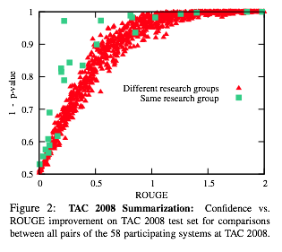
A quick note on Berg-Kirkpatrick et al EMNLP-2012, “An Empirical Investigation of Statistical Significance in NLP”. They make lots of graphs of p-values against observed magnitudes and talk about “curves”, e.g.

We see the same curve-shaped trend we saw for summarization and dependency parsing. Different group comparisons, same group comparisons, and system combination comparisons form distinct curves.

For example, Figure 2.

I fear they made 10 graphs to rediscover a basic statistical fact: a p-value comes from a null hypothesis CDF. That’s what these “curve-shaped trends” are in all their graphs. They are CDFs.

To back up, the statistical significance testing question is whether, in their notation, the observed dataset performance difference \(\delta(x)\) is “real” or not: if you were to resample the data, how much would \(\delta(x)\) vary? One way to think about significance testing in this setting is, it asks if the difference you got has the same sign as the true difference. (not quite the Bayesian posterior of what Gelman et al call a “sign error”, but rather a kind of pessimistic worst-case probability of it; this is how classic hypothesis testing works.) Getting the sign right is an awfully minimal requirement of whether your results are important, but seems useful to do.

Strip away all the complications of bootstrap tests and stupidly overengineered NLP metrics, and consider the simple case where, in their notation, the observed dataset difference \( \delta(x) \) is a simple average of per-unit differences \(\delta(one unit)\); i.e. per-sentence, per-token, per-document, whatever. The standard error is the standard deviation of the dataset difference, a measure of how much it were to vary if the units were resampled, and unit-level differences were i.i.d. This standard error is, according to bog-standard Stat 101 theory,

\[ \sqrt{Var(\delta(x))} = \frac{\sqrt{Var(\delta(\text{one unit}))} }{ \sqrt{n} } \]

And you get 5% significance (in a z-test.. is this a “paired z-test”?) if your observed difference \(\delta(x)\) is more than 1.96 times its standard error. The number 1.96 comes from the normal CDF. In particular, you can directly evaluate your p-value via, in their notation again,

\[ pvalue(x) = 1-NormCDF\left(
\delta(x);\ \
mean=0,\ sd=\frac{\sqrt{Var(\delta(\text{one unit}))} }{ \sqrt{n} }
\right)
\]

(I think I wrote a one-sided test there.) The point is you can read off, from the standard error equation, the important determinants of significance: (numerator) the variability of system performance, variability between systems, and difficulty of the task; and (denominator) the size of the dataset. You shouldn’t need to read this paper to know the answer is “no” to the qustion Is it true that for each task there is a gain which roughly implies significance?

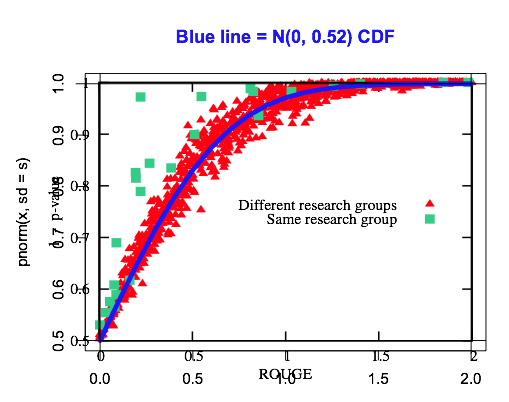
In fact, lots of their graphs look an awful lot like a normal CDF. For example, here is Figure 2 again, where I’ve plotted a normal CDF on top. (Yes, copy and pasted from R.) They’re plotting \(1-pvalue\), which is the null hypothesis CDF. Indeed, for the red points they look pretty similar:

Now, they’re using bootstrap tests, which are great and in principle better than the z-test because they can handle all sorts of nasty, non-analyzable metrics like BLEU, and there are some subtleties with comparing all pairs of systems I admit I didn’t totally follow. (There’s another point that BLEU should have been designed to be mathematically simpler to analyze, instead of all that crap with global penalties, though the stupid overengineering of NLP metrics is a topic for another blog post.) But in nonparametric tests there’s still a null hypothesis CDF — it’s the ECDF of the statistic over simulation outcomes — and your pvalue comes from it! I think this is what all those curves are they claim to have discovered. Every dataset has its own null hypothesis CDF; if it was the normal approximation case, those factors go into the numerator and denominator of the standard error. (If you want to read more about the empirical CDF plug-in estimator explanation of these nonparametric tests, see the wonderful chapters 6 to 7 to 10 or so of Larry Wasserman’s All of Statistics.)

In fact, if their recovered null hypothesis CDFs really are the same as an unpaired z-test’s null hypothesis CDF, that could be telling is that these NLP metrics are truly overengineered: their statistical variability behaves similarly to an arithmetic mean. That’s a not a for-sure conclusion based on the data they show, but perhaps worth thinking about.

The more interesting thing about Figure 2 are those points in green off the null hypo CDF curve. At first when I saw it I got excited because I thought they were going to claim evidence of self-serving reporting biases, like some people have done for various classes of experimental papers (via p-value histograms across papers and such, e.g. Vul et al’s “Voodoo Correlations” paper.) But actually, they say it’s just an example of paired testing at work: the same research group will produce a series of systems that have very highly correlated outputs; this is a textbook example of where paired tests have greater statistical power than unpaired ones, since they have the ability to only pay attention to pairs where things changed, and not let those differences be washed out by all the pairs that haven’t changed. Well, maybe. Someone should investigate potential “voodoo performance differences”. Now that would be an exciting NLP methodology paper.

The last section, basically a demonstration that “statistical significance != substantive significance” in the context of parsing (where practically you might care about domains other than the late-1980′s Wall Street Journal, which has been presumably over-optimized via 15 years and zillions of PhD theses’ worth of effort), was nice. Since statistical signicance testing is basically the question “Do I have the correct sign of the performance difference?”, the question “Is my performance difference important?” is obviously a whole other thing. You probably need to get the former right before confidently answering the latter, but anyone who runs a significance test and mindlessly declares victory is hiding behind the former to dodge the latter.

This paper illustrates the point in an odd fashion, looking at the out-of-domain p-value versus in-domain p-value — why not just directly map between domain effect sizes instead of doing everything roundabout with significance tests, which hide what’s truly going on? For example, just plot Brown performance versus WSJ performance, and throw in standard error bars if you like. (I guess if you’re a true NLP engineer, you always care about paired tests since it makes it easier to see incremental system improvements, thus the general focus on hypothesis tests instead of confidence regions? I like confidence regions and standard errors much more as a thing to be reported, you can trivially read off unpaired tests from them yourself, but you don’t get the increased power of paired testing then.)

But it’s still a good point. I feel like anyone who’s done real-world NLP is used to the fact that academic NLP research is often horribly insular and narrowly focused, and would not be surprised at all about results that WSJ performance is more weakly correlated with out-of-domain performance than, well, WSJ performance; but maybe it’s worth communicating this to the academic NLP audience.

p.s. sorry to harp on this but the unfortunately failed-to-be-cited Clark et al. ACL 2011 is really relevant. In that paper they actually break out different sources of variability for the specific problem of variability due to optimizer instability.