Memorizing small tables


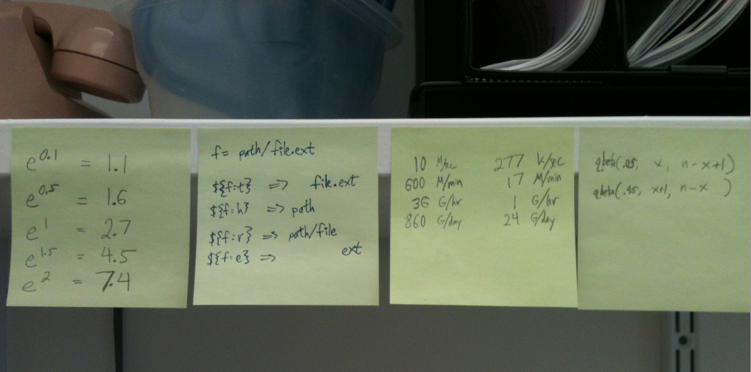
Lately, I’ve been trying to memorize very small tables, especially for better intuitions and rule-of-thumb calculations. At the moment I have these above my desk:

The first one is a few entries in a natural logarithm table. There are all these stories about how in the slide rule era, people would develop better intuitions about the scale of logarithms because they physically engaged with them all the time. I spend lots of time looking at log-likelihoods, log-odds-ratios, and logistic regression coefficients, so I think it would be nice to have quick intuitions about what they are. (Though the Gelman and Hill textbook has an interesting argument against odds scale interpretations of logistic regression coefficients.)

The second one are some zsh filename manipulation shortcuts. OK, this is more narrow than the others, but pretty useful for me at least.

The third one are rough unit equivalencies for data rates over time. I find this very important for quickly determining whether a long-running job is going to take a dozen minutes, or a few hours, or a few days. In particular, many data transfer commands (scp, wget, s3cmd) immediately tell you a rate per second, which you then can scale up. (And if you’re using a CPU-bound pipeline command, you can always use the amazing pv command to get a rate-per-second estimate.) This table is inspired by the “Numbers Everyone Should Know” list.

The fourth one is the Clopper-Pearson binomial confidence interval. Actually, the more useful ones to memorize are Wald binomial intervals, which are easy because they’re close to \(\pm 1/\sqrt{n}\). Good party trick. This sticky is actually the relevant R calls (type binom.test and press enter); I was using small-n binomial hypothesis testing a lot recently so wanted to get more used to it. Maybe this one isn’t very useful.
5 Comments

Be careful with dictionary-based text analysis

OK, everyone loves to run dictionary methods for sentiment and other text analysis — counting words from a predefined lexicon in a big corpus, in order to explore or test hypotheses about the corpus. In particular, this is often done for sentiment analysis: count positive and negative words (according to a sentiment polarity lexicon, which was derived from human raters or previous researchers’ intuitions), and then proclaim the output yields sentiment levels of the documents. More and more papers come out every day that do this. I’ve done this myself. It’s interesting and fun, but it’s easy to get a bunch of meaningless numbers if you don’t carefully validate what’s going on. There are certainly good studies in this area that do further validation and analysis, but it’s hard to trust a study that just presents a graph with a few overly strong speculative claims as to its meaning. This happens more than it ought to.

I was happy to see a similarly critical view in a nice working paper by Justin Grimmer and Brandon Stewart, Text as Data: The Promise and Pitfalls of Automatic Content Analysis Methods for Political Texts.

Since I think these arguments need to be more widely known, here’s a long quote from Section 4.1 … see also the paper for more details (and lots of other interesting stuff). Emphases are mine.

For dictionary methods to work well, the scores attached to words must closely align with how the words are used in a particular context. If a dictionary is developed for a specific application, then this assumption should be easy to justify. But when dictionaries are created in one substantive area and then applied to another problems, serious errors can occur. Perhaps the clearest example of this is shown in Loughran and McDonald (2011). Loughran and McDonald (2011) critique the increasingly common use of off the shelf dictionaries to measure the tone of statutorily required corporate earning reports in the accounting literature. They point out that many words that have a negative connotation in other contexts, like tax, cost, crude (oil) or cancer, may have a positive connotation in earning reports. For example, a health care company may mention cancer often and oil companies are likely to discuss crude extensively. And words that are not identified as negative in off the shelf dictionaries may have quite negative connotation in earning reports (unanticipated, for example).

Dictionaries, therefore, should be used with substantial caution. Scholars must either explicitly establish that word lists created in other contexts are applicable to a particular domain, or create a problem specific dictionary. In either instance, scholars must validate their results. But measures from dictionaries are rarely validated. Rather, standard practice in using dictionaries is to assume the measures created from a dictionary are correct and then apply them to the problem. This is due, in part, to the exceptional difficulties in validating dictionaries. Dictionaries are commonly used to establish granular scales of a particular kind of sentiment, such as tone. While this is useful for applications, the granular measures insure that it is essentially impossible to derive gold standard evaluations based on human coding of documents, because of the difficulty of establishing reliable granular scales from humans (Krosnick, 1999).

The consequence of domain specificity and lack of validation is that most analyses based on dictionaries are built on shaky foundations. Yes, dictionaries are able to produce measures that are claimed to be about tone or emotion, but the actual properties of these measures – and how they relate to the concepts their attempting to measure – are essentially a mystery. Therefore, for scholars to effectively use dictionary methods in their future work, advances in the validation of dictionary methods must be made. We suggest two possible ways to improve validation of dictionary methods. First, the classification problem could be simplified. If scholars use dictionaries to code documents into binary categories (positive or negative tone, for example), then validation based on human gold standards and the methods we describe in Section 4.2.4 is straightforward. Second, scholars could treat measures from dictionaries similar to how we validations from unsupervised methods are conducted (see Section 5.5). This would force scholars to establish that their measures of underlying concepts have properties associated with long standing expectations.

And after an example analysis,

… we reiterate our skepticism of dictionary based measures. As is standard in the use of dictionary measures (for example, Young and Soroka (2011)) the measures are presented here without validation. This lack of validation is due in part because it is exceedingly difficult to demonstrate that our scale of sentiment precisely measures differences in sentiment expressed towards Russia. Perhaps this is because it is equally difficult to define what would constitute these differences in scale.

2 Comments

Information theory stuff


Actually this post is mainly to test the MathJax installation I put into WordPress via this plugin. But information theory is great, why not?

The probability of a symbol is \(p\).

It takes \(\log \frac{1}{p} = -\log p\) bits to encode one symbol — sometimes called its “surprisal”. Surprisal is 0 for a 100% probable symbol, and ranges up to \(\infty\) for extremely low probability symbols. This is because you use a coding scheme that encodes common symbols as very short strings, and less common symbols as longer ones. (e.g. Huffman or arithmetic coding.) We should say logarithms are base-2 so information is measured in bits.\(^*\)

If you have a stream of such symbols and a probability distribution \(\vec{p}\) for them, where a symbol \(i\) comes at probability \(p_i\), then the average message size is the expected surprisal:

\[ H(\vec{p}) = \sum_i p_i \log \frac{1}{p_i} \]

this is the Shannon entropy of the probability distribution \( \vec{p} \), which is a measure of its uncertainty. In fact, if you start with a few pretty reasonable axioms for how to design a measurement of uncertainty of a discrete probability distribution, you end up with the above equation as the only possible measure. (I think. This is all in Shannon’s original paper.)

Now, what if you have symbols at a distribution \( \vec{p} \) but you encode then with the wrong distribution \( \vec{q} \)? You pay \(\log\frac{1}{q}\) bits per symbol but the expectation is under the true distribution \(\vec{p}\). Then the average message size is called the cross-entropy between the distributions:

\[ H(\vec{p},\vec{q}) = \sum_i p_i \log \frac{1}{q_i} \]

How much worse is this coding compared to the optimal one? (I.e. how much a cost do you pay for encoding with the wrong distribution?) The optimal one is size \( \sum -p_i \log p_i \) so it’s just

\[ \begin{align}
& \sum_i -p_i \log q_i + p_i \log p_i \\
KL(\vec{p} || \vec{q})=
&\sum_i p_i \log \frac{p_i}{q_i}
\end{align} \]

which is called the relative entropy or Kullback-Leibler divergence, and it’s a measurement of the disssimilarity of the distributions \(\vec{p}\) and \(\vec{q}\). You can see it’s about dissimilarity because if \(\vec{p}\) and \(\vec{q}\) were the same, then the inner term \(\log\frac{p}{q}\) would always be 0 and the whole thing comes out to be 0.

For more, I rather like the early chapters of the free online textbook by David MacKay: “Information Theory, Inference, and Learning Algorithms”. That’s where I picked up the habit of saying surprisal is \( \log \frac{1}{p} \) instead of \(-\log p\); the former seems more intuitive to me, and then you don’t have a pesky negative sign in the entropy and cross-entropy equations. In general the book is great at making things intuitive. Its main weakness is you can’t trust the insane negative things he says about frequentist statistics, but that’s another discussion.

\(^*\) You can use natural logs or whatever and it’s just different sized units: “nats”, as you can see in the fascinating Chapter 18 of MacKay on codebreaking, which features Bletchley Park, Alan Turing, and Nazis.

5 Comments

End-to-end NLP packages

What freely available end-to-end natural language processing (NLP) systems are out there, that start with raw text, and output parses and semantic structures? Lots of NLP research focuses on single tasks at a time, and thus produces software that does a single task at a time. But for various applications, it is nicer to have a full end-to-end system that just runs on whatever text you give it.

If you believe this is a worthwhile goal (see caveat at bottom), I will postulate there aren’t a ton of such end-to-end, multilevel systems. Here are ones I can think of. Corrections and clarifications welcome.

  • Stanford CoreNLP. Raw text to rich syntactic dependencies (LFG-inspired). Also POS, NER, coreference.
  • C&C tools. From (sentence-segmented, tokenized?) text to rich syntactic dependencies (CCG-based) and also a semantic representation. POS and chunks on the way. Does anyone use this much? It seems underappreciated relative to its richness.
  • Senna. Sentence-segmented text -> parse trees, plus POS, NER, chunks, and semantic role labeling. This one is quite new; is it as good? It doesn’t give syntactic dependencies, though for some applications semantic role labeling is similar or better (or worse?). I’m a little concerned that its documentation seems overly focused on competing in evaluation datasets, as opposed to trying to ensure they’ve made something more broadly useful. (To be fair, they’re focused on developing algorithms that could be broadly applicable to different NLP tasks; that’s a whole other discussion.)

If you want to quickly get some sort of shallow semantic relations, a.k.a. high-level syntactic relations, one of the above packages might be your best bet. Are there others out there?

Restricting oneself to these full end-to-end systems is also funny since you can mix-and-match components to get better results for what you want. One example: if you have constituent parse trees and want dependencies, you could swap in the Stanford Dependency extractor (or another one like pennconverter?) to post-process the parses. Or you could swap in the Charniak-Johnson or Berkeley parser into the middle of the Stanford CoreNLP stack. Or you could use a direct dependency parser (I think Malt is the most popular?) and skip the pharse structure step. Etc.

It’s worth noting several other NLP libraries that I see used a lot. I believe that, unlike the above, they don’t focus on out-of-the-box end-to-end NLP analysis (though you can certainly use them to perform various parts of an NLP pipeline).

  • OpenNLP — I’ve never used it but lots of people like it. Seems well-maintained now? Does chunking, tagging, even coreference.
  • LingPipe — has lots of individual algorithms and high-quality implementations. Only chunking and tagging (I think). It’s only quasi-free.
  • Mallet — focuses on information extraction and topic modeling, so slightly different than the other packages listed here.
  • NLTK — I always have a hard time telling what this actually does, compared to what it aims to teach you to do. It seems to do various tagging and chunking tasks. I use the nltk_data.zip archive all the time though (I can’t find a direct download link unfortunately), for its stopword lists and small toy corpora. (Including the Brown Corpus! I guess it now counts as a toy corpus since you can grep it in less than a second.)

These packages are nice in terms of documentation and software engineering, but they don’t do any syntactic parsing or other shallow relational extraction. (NLTK has some libraries that appear to do parsing and semantics, but it’s hard to tell how serious they are.)

Oh finally, there’s also UIMA, which isn’t really a tool, but rather a high-level API to integrate together your tools. GATE also heavily emphasizes the framework aspect, but does come with some sort of tools.

19 Comments

CMU Twitter Part-of-Speech tagger 0.2

Announcement: We recently released a new version (0.2) of our part-of-speech tagger for English Twitter messages, along with annotations and interface. See the link for more details.

Leave a comment

One last thing on the Norvig vs. Chomsky thing from a little while ago (http://norvig.com/chomsky.html), which (correctly) casts the issue as Shannon vs. Chomsky.

The relevant seminal publications are:

  • Shannon, “Mathematical Theory of Communication,” 1948
  • Chomsky, “Syntactic Structures,” 1957

One of those historical figures is still around and representing himself in 2011 — he should get credit just for still showing up to the fight. Are there any historical figures from the Shannon side still around?  What I would’ve given to see a Jelinek vs. Chomsky public debate.  Though I guess Pereira vs. Chomsky would be pretty great.

3 Comments

Good linguistic semantics textbook?

I’m looking for recommendations for a good textbook/handbook/reference on (non-formal) linguistic semantics.  My undergrad semantics course was almost entirely focused on logical/formal semantics, which is fine, but I don’t feel familiar with the breadth of substantive issues — for example, I’d be hard-pressed to explain why something like semantic/thematic role labeling should be useful for anything at all.

I somewhat randomly stumbled upon Frawley 1992 (review) in a used bookstore and it seemed pretty good — in particular, it cleanly separates itself from the philosophical study of semantics, and thus identifies issues that seem amenable to computational modeling.

I’m wondering what else is out there?  Here’s a comparison of three textbooks.

5 Comments

How much text versus metadata is in a tweet?

This should have been a blog post, but I got lazy and wrote a plaintext document instead.

For twitter, context matters: 90% of a tweet is metadata and 10% is text.  That’s measured by (an approximation of) information content; by raw data size, it’s 95/5.

2 Comments

iPhone autocorrection error analysis

re @andrewparker:

My iPhone auto-corrected “Harvard” to “Garbage”. Well played Apple engineers.

I was wondering how this would happen, and then noticed that each character pair has 0 to 2 distance on the QWERTY keyboard.  Perhaps their model is eager to allow QWERTY-local character substitutions.

>>> zip(‘harvard’,'garbage’)
[('h', 'g'), ('a', 'a'), ('r', 'r'), ('v', 'b'), ('a', 'a'), ('r', 'g'), ('d', 'e')]

And then most any language model thinks p(“garbage”) > p(“harvard”), at the very least in a unigram model with a broad domain corpus.  So if it’s a noisy channel-style model, they’re underpenalizing the edit distance relative to the LM prior. (Reference: Norvig’s noisy channel spelling correction article.)

On the other hand, given how insane iPhone autocorrections are, and from the number of times I’ve seen it delete a quite reasonable word I wrote, I’d bet “harvard” isn’t even in their LM.  (Where the LM is more like just a dictionary; call it quantizing probabilities to 1 bit if you like.)  I think Hal mentioned once he would gladly give up GB’s of storage for a better language model to make iPhone autocorrect not suck.  That sounds like the right tradeoff to me.

Language models with high coverage are important.  As illustrated in e.g. one of those Google MT papers.  Wish Apple would figure this out too.

6 Comments

Log-normal and logistic-normal terminology

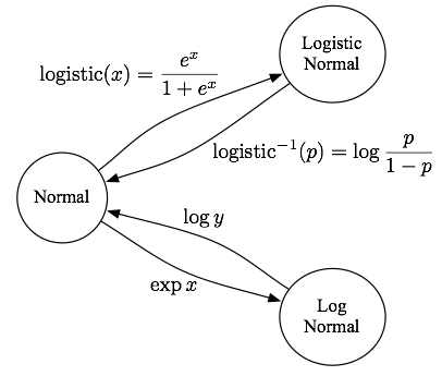
I was cleaning my office and found a back-of-envelope diagram Shay drew me once, so I’m writing it up to not forget.  The definitions of the logistic-normal and log-normal distributions are a little confusing with regard to their relationship to the normal distribution.  If you draw samples from one, the arrows below show the transformation to make it such you have samples from another.

For example, if x ~ Normal, then transforming as y=exp(x) implies y ~ LogNormal.  The adjective terminology is inverted: the logistic function goes from normal to logistic-normal, but the log function goes from log-normal to normal (other way!).  The log of the log-normal is normal, but it’s the logit of the logistic normal that’s normal.

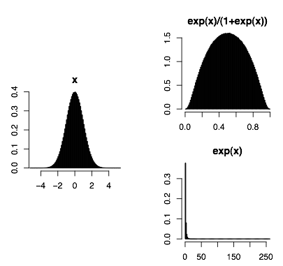
Here are densities of these different distributions via transformations from a standard normal.

In R:  x=rnorm(1e6); hist(x); hist(exp(x)/(1+exp(x)); hist(exp(x))

Just to make things more confusing, note the logistic-normal distribution is completely different than the logistic distribution.

What are these things?  There’s lots written online about log-normals.  Neat fact: it arises from lots of multiplicative effects (by the CLT, since additive effects imply the normal).  The very nice Clauset et al. (slidesblogpost) finds log-normals and stretched exponentials fit pretty well to many types of data that are often claimed to be power-law.

The logistic-normal is more obscure–it doesn’t even have a Wikipedia page, so see the original Aitchison and Shen.  Hm, on page 2 they talk about the log-normal, so they’re responsible for the very slight naming weirdness.  The logistic-normal is a useful Bayesian prior for multinomial distributions, since in the d-dimensional multivariate case it defines a probability distribution over the simplex (i.e. parameterizations of d-dim. multinomials), similar to the Dirichlet, but you can capture covariance effects and chain them together and other fun things, though inference can be trickier (typically via variational approximations).  A biased sample of text modeling examples include Blei and Lafferty, another B&L, Cohen and Smith, Eisenstein et al.

OK, so maybe these distributions aren’t really related beyond involving transformations of the normal.

Finally, note that the diagram only writes out the logistic-normal for the one-dimensional case; in the multivariate case, there’s an additional wrinkle that the logistic-normal has one less dimension than the normal, since you don’t need a parameter for the last one dimension (subtract the rest out of 1).  For example, a 3-d normal (distribution over 3-space) corresponds to a logistic-normal distribution over a simplex in 3-space, having only 2 dimensions.

4 Comments