Berkeley SDA and the General Social Survey

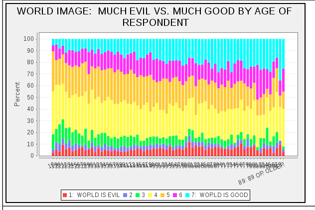
It is worth contemplating how grand the General Social Survey is. When playing around with the Statwing YC demo (which is very cool!) I was reminded of the very old-school SDA web tool for exploratory cross-tabulation analyses… They have the GSS loaded and running here. The GSS is so large you can analyze really weird combinations of variables. For example, here is one I just did: How much good versus evil is there in the world (on a 7 point scale, of course!), versus age.

2 Comments

Re

The best I can do is: I once programmed Prolog, wrapped inside Tcl and Ruby, to generate a query against a C++ IR engine, which generated features for a boosted decision tree trained in R, to rank documents indexed with that segfault-prone Tcl/Prolog/C system wrapped in Java/Hadoop. Then I wrote a Javascript/Ruby web interface on top.

Switching between these languages is too much for one days’ work. Educational, but not the best way to do things.

1 Comment

p-values, CDF’s, NLP etc.

Update Aug 10: THIS IS NOT A SUMMARY OF THE WHOLE PAPER! it’s whining about one particular method of analysis before talking about other things further down


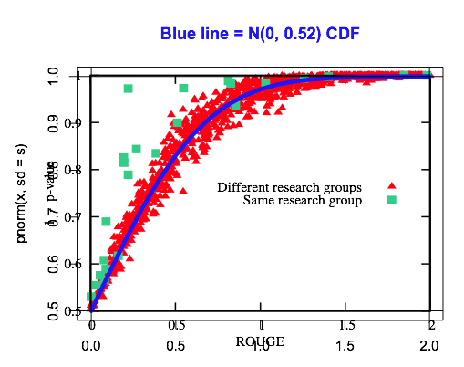
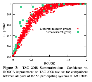
A quick note on Berg-Kirkpatrick et al EMNLP-2012, “An Empirical Investigation of Statistical Significance in NLP”. They make lots of graphs of p-values against observed magnitudes and talk about “curves”, e.g.

We see the same curve-shaped trend we saw for summarization and dependency parsing. Different group comparisons, same group comparisons, and system combination comparisons form distinct curves.

For example, Figure 2.

I fear they made 10 graphs to rediscover a basic statistical fact: a p-value comes from a null hypothesis CDF. That’s what these “curve-shaped trends” are in all their graphs. They are CDFs.

To back up, the statistical significance testing question is whether, in their notation, the observed dataset performance difference \(\delta(x)\) is “real” or not: if you were to resample the data, how much would \(\delta(x)\) vary? One way to think about significance testing in this setting is, it asks if the difference you got has the same sign as the true difference. (not quite the Bayesian posterior of what Gelman et al call a “sign error”, but rather a kind of pessimistic worst-case probability of it; this is how classic hypothesis testing works.) Getting the sign right is an awfully minimal requirement of whether your results are important, but seems useful to do.

Strip away all the complications of bootstrap tests and stupidly overengineered NLP metrics, and consider the simple case where, in their notation, the observed dataset difference \( \delta(x) \) is a simple average of per-unit differences \(\delta(one unit)\); i.e. per-sentence, per-token, per-document, whatever. The standard error is the standard deviation of the dataset difference, a measure of how much it were to vary if the units were resampled, and unit-level differences were i.i.d. This standard error is, according to bog-standard Stat 101 theory,

\[ \sqrt{Var(\delta(x))} = \frac{\sqrt{Var(\delta(\text{one unit}))} }{ \sqrt{n} } \]

And you get 5% significance (in a z-test.. is this a “paired z-test”?) if your observed difference \(\delta(x)\) is more than 1.96 times its standard error. The number 1.96 comes from the normal CDF. In particular, you can directly evaluate your p-value via, in their notation again,

\[ pvalue(x) = 1-NormCDF\left(
\delta(x);\ \
mean=0,\ sd=\frac{\sqrt{Var(\delta(\text{one unit}))} }{ \sqrt{n} }
\right)
\]

(I think I wrote a one-sided test there.) The point is you can read off, from the standard error equation, the important determinants of significance: (numerator) the variability of system performance, variability between systems, and difficulty of the task; and (denominator) the size of the dataset. You shouldn’t need to read this paper to know the answer is “no” to the qustion Is it true that for each task there is a gain which roughly implies significance?

In fact, lots of their graphs look an awful lot like a normal CDF. For example, here is Figure 2 again, where I’ve plotted a normal CDF on top. (Yes, copy and pasted from R.) They’re plotting \(1-pvalue\), which is the null hypothesis CDF. Indeed, for the red points they look pretty similar:

Now, Continue reading

3 Comments

The $60,000 cat: deep belief networks make less sense for language than vision

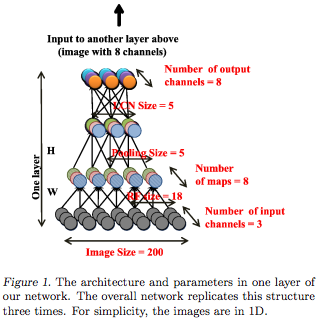
There was an interesting ICML paper this year about very large-scale training of deep belief networks (a.k.a. neural networks) for unsupervised concept extraction from images. They (Quoc V. Le and colleagues at Google/Stanford) have a cute example of learning very high-level features that are evoked by images of cats (from YouTube still-image training data); one is shown below.

For those of us who work on machine learning and text, the question always comes up, why not DBN’s for language? Many shallow latent-space text models have been quite successful (LSI, LDA, HMM, LPCFG…); there is hope that some sort of “deeper” concepts could be learned. I think this is one of the most interesting areas for unsupervised language modeling right now.

But note it’s a bad idea to directly analogize results from image analysis to language analysis. The problems have radically different levels of conceptual abstraction baked-in. Consider the problem of detecting the concept of a cat; i.e. those animals that meow, can be our pets, etc. I hereby propose a system that can detect this concept in text, and compare it to the image analysis DBN as follows.

Problem

Concept representation

Concept detector

Cost to create concept detector

Image analysis

1,152,000 CPU-hours to train neural network

$61,056 at current GCE prices

Language analysis


cat

a.k.a.
1100011
1100001
1110100

"cat" in 
re.split('[^a-z]', text.lower())
147 CPU-microseconds to compile finite-state network /[^a-z]/

$0.000078 at GCE prices

I mean: you can identify the concept “cat” by tokenizing a text, i.e. breaking it up into words, and looking for the word “cat”. To identify the “cat” concept from a vector of pixel intensities, you have to run through a cascade of filters, edge detectors, shape detectors and more. This paper creates the image analyzer with tons of unsupervised learning; in other approaches you still have to train all the components in your cascade. [Note.]

In text, the concept of “cat” is immediately available on the surface — there’s a whole word for it. Think of all the different shapes and types of cats which you could call a “cat” and be successfully understood. Words are already a massive dimension reduction of the space of human experiences. Pixel intensity vectors are not, and it’s a lot of work to reduce that dimensionality. Our vision systems are computational devices that do this dimension reduction, and they took many millions of years of evolution to construct.

In comparison, the point of language is communication, so it’s designed, at least a little bit, to be comprehensible — pixel intensity vectors do not seem to be have such a design goal. ["Designed."] The fact that it’s easy to write a rule-based word extractor with /[^a-zA-Z0-9]/ doesn’t mean bag-of-words or n-grams are “low-level”; it just means that concept extraction is easy with text. In particular, English has whitespace conventions and simple enough morphology that you can write a tokenizer by hand, and we’ve designed character encoding standards let computers unambiguously map between word forms and binary representations.

Unsupervised cross-lingual phonetic and morphological learning is closer, cognitive-level-of-abstraction-wise, to what the deep belief networks people are trying to do with images. To make a fairer table above, you might want to compare to the training time of an unsupervised word segmenter / cross-lingual lexicon learner.

[Another aside: The topic modeling community, in particular, seems to often mistakenly presume you need dimension reduction to do anything with text. Every time you run a topic model you're building off of your rule-based concept extractor -- your tokenizer -- which might very well be doing all the important work. Don't forget you can sometimes get great results with just the words (and phrases!), for both predictive and exploratory tasks. Getting topics can also be great, but it would be nice to have a better understanding exactly when or how they're useful.]

This isn’t to say that lexicalized models (be they document or sequence-level) aren’t overly simple or crude. Just within lexical semantics, it’s easy to come up with examples of concepts that “cat” might refer to, but you want other words as well. You could have synonyms {cat, feline}, or refinements {cat, housecat, tabby} or generalizations {cat, mammal, animal} or things that seem related somehow but get tricky the more you think about it {cat, tiger, lion}. Or maybe the word “cat” is a part of a broad topical constellation of words {cat, pets, yard, home} or with an affective aspect twist {cat, predator, cruel, hunter} or maybe a pretty specific narrative frame {cat, tree, rescue, fireman}. (I love how ridiculous this last example is, but we all instantly recognize the scenario it evokes. Is this an America-specific cultural thing?)

If you want to represent and differentiate between the concepts evoked by these wordsets, then yes, the bare symbol “cat” is too narrow (or too broad), and maybe we want something “deeper”. So what does “deep learning” mean? There’s a mathematical definition in the largeness of the class of functions these models can learn; but practically when you’re running these things, you need a criterion for how good of concepts you’re learning, which I think the rhetoric of “deep learning” is implicitly appealing to.

In the images case, “deep” seems to mean “recognizable concepts that look cool”. (There’s room to be cynical about this, but I think it’s fine when you’re comparing to things that are not recognizable.) In the text case, if you let yourself use word-and-ngram extraction, then you’ve already started with recognizable concepts — where are you going next? (And how do you evaluate?) One interesting answer is, let’s depart lexical semantics and go compositional; but perhaps there are many possibilities.


Note on table: Timing of regex compilation was via IPython %timeit re.purge();re.compile(‘[^a-z]‘). Also I’m excluding human costs — hundreds (thousands?) of hours from 8 CS researcher coauthors (and imagine how much Ng and Dean cost in dollars!), versus whatever skill level it is to write a regex. The former costs are justified given it is, after all, research; the regex works well because someone invented all the regular expression finite-state algorithms we now take for granted. But there are awfully good reasons there was so much finite-state research decades ago: they’re really, really useful for processing symbolic systems created by humans; most obviously artificial programming languages designed that way, but also less strict quasi-languages like telephone number formats, and certain natural language analysis tasks like tokenization and morphology…

“Design:” …where we can define “design” and “intention” in a Herbert Simon sort of way to mean “part of the optimization objective of either cultural or biological evolution”; i.e. aspects of language that don’t have good communicative utility might be go away over time, but the processes that that give us light patterns hitting our retina are quite exogenous, modulo debates about God or anthropic principles etc.

3 Comments

F-scores, Dice, and Jaccard set similarity

The Dice similarity is the same as F1-score; and they are monotonic in Jaccard similarity. I worked this out recently but couldn’t find anything about it online so here’s a writeup.

Let \(A\) be the set of found items, and \(B\) the set of wanted items. \(Prec=|AB|/|A|\), \(Rec=|AB|/|B|\). Their harmonic mean, the \(F1\)-measure, is the same as the Dice coefficient:
\begin{align*}
F1(A,B)
&= \frac{2}{1/P+ 1/R}
= \frac{2}{|A|/|AB| + |B|/|AB|} \\
Dice(A,B)
&= \frac{2|AB|}{ |A| + |B| } \\
&= \frac{2 |AB|}{ (|AB| + |A \setminus B|) + (|AB| + |B \setminus A|)} \\
&= \frac{|AB|}{|AB| + \frac{1}{2}|A \setminus B| + \frac{1}{2} |B \setminus A|}
\end{align*}

It’s nice to characterize the set comparison into the three mutually exclusive partitions \(AB\), \(A \setminus B\), and \(B \setminus A\). This illustrates Dice’s close relationship to the Jaccard metric,
\begin{align*}
Jacc(A,B)
&= \frac{|AB|}{|A \cup B|} \\
&= \frac{|AB|}{|AB| + |A \setminus B| + |B \setminus A|}
\end{align*}
And in fact \(J = D/(2-D)\) and \(D=2J/(1+J)\) for any input, so they are monotonic in one another.
The Tversky index (1977) generalizes them both,
\begin{align*}
Tversky(A,B;\alpha,\beta)
&= \frac{|AB|}{|AB| + \alpha|A\setminus B| + \beta|B \setminus A|}
\end{align*}
where \(\alpha\) and \(\beta\) control the magnitude of penalties of false positive versus false negative errors. It’s easy to work out that all weighted F-measures correspond to when \(\alpha+\beta=1\). The Tversky index just gives a spectrum of ways to normalize the size of a two-way set intersection. (I always thought Tversky’s more mathematical earlier work (before the famous T&K heuristics-and-biases stuff) was pretty cool. In the 1977 paper he actually does an axiomatic derivation of set similarity measures, though as far as I can tell this index doesn’t strictly derive from them. Then there’s a whole debate in cognitive psych whether similarity is a good way to characterize reasoning about objects but that’s another story.)

So you could use either Jaccard or Dice/F1 to measure retrieval/classifier performance, since they’re completely monotonic in one another. Jaccard might be a little unintuitive though, because it’s always less than or equal min(Prec,Rec); Dice/F is always in-between.

2 Comments

Cosine similarity, Pearson correlation, and OLS coefficients

Cosine similarity, Pearson correlations, and OLS coefficients can all be viewed as variants on the inner product — tweaked in different ways for centering and magnitude (i.e. location and scale, or something like that).

Details:

You have two vectors \(x\) and \(y\) and want to measure similarity between them. A basic similarity function is the inner product

\[ Inner(x,y) = \sum_i x_i y_i = \langle x, y \rangle \]

If x tends to be high where y is also high, and low where y is low, the inner product will be high — the vectors are more similar.

The inner product is unbounded. One way to make it bounded between -1 and 1 is to divide by the vectors’ L2 norms, giving the cosine similarity

\[ CosSim(x,y) = \frac{\sum_i x_i y_i}{ \sqrt{ \sum_i x_i^2} \sqrt{ \sum_i y_i^2 } }
= \frac{ \langle x,y \rangle }{ ||x||\ ||y|| }
\]

This is actually bounded between 0 and 1 if x and y are non-negative. Cosine similarity has an interpretation as the cosine of the angle between the two vectors; you can illustrate this for vectors in \(\mathbb{R}^2\) (e.g. here).

Cosine similarity is not invariant to shifts. If x was shifted to x+1, the cosine similarity would change. What is invariant, though, is the Pearson correlation. Let \(\bar{x}\) and \(\bar{y}\) be the respective means:

\begin{align}
Corr(x,y) &= \frac{ \sum_i (x_i-\bar{x}) (y_i-\bar{y}) }{
\sqrt{\sum (x_i-\bar{x})^2} \sqrt{ \sum (y_i-\bar{y})^2 } }
\\
& = \frac{\langle x-\bar{x},\ y-\bar{y} \rangle}{
||x-\bar{x}||\ ||y-\bar{y}||} \\
& = CosSim(x-\bar{x}, y-\bar{y})
\end{align}

Correlation is the cosine similarity between centered versions of x and y, again bounded between -1 and 1. People usually talk about cosine similarity in terms of vector angles, but it can be loosely thought of as a correlation, if you think of the vectors as paired samples. Unlike the cosine, the correlation is invariant to both scale and location changes of x and y.

This isn’t the usual way to derive the Pearson correlation; usually it’s presented as a normalized form of the covariance, which is a centered average inner product (no normalization)

\[ Cov(x,y) = \frac{\sum (x_i-\bar{x})(y_i-\bar{y}) }{n}
= \frac{ \langle x-\bar{x},\ y-\bar{y} \rangle }{n} \]

Finally, these are all related to the coefficient in a one-variable linear regression. For the OLS model \(y_i \approx ax_i\) with Gaussian noise, whose MLE is the least-squares problem \(\arg\min_a \sum (y_i – ax_i)^2\), a few lines of calculus shows \(a\) is

\begin{align}
OLSCoef(x,y) &= \frac{ \sum x_i y_i }{ \sum x_i^2 }
= \frac{ \langle x, y \rangle}{ ||x||^2 }
\end{align}

This looks like another normalized inner product. But unlike cosine similarity, we aren’t normalizing by \(y\)’s norm — instead we only use \(x\)’s norm (and use it twice): denominator of \(||x||\ ||y||\) versus \(||x||^2\).

Not normalizing for \(y\) is what you want for the linear regression: if \(y\) was stretched to span a larger range, you would need to increase \(a\) to match, to get your predictions spread out too.

Often it’s desirable to do the OLS model with an intercept term: \(\min_{a,b} \sum (y – ax_i – b)^2\). Then \(a\) is

\begin{align}
OLSCoefWithIntercept(x,y) &= \frac
{ \sum (x_i – \bar{x}) y_i }
{ \sum (x_i – \bar{x})^2 }
= \frac{\langle x-\bar{x},\ y \rangle}{||x-\bar{x}||^2}
\\
&= OLSCoef(x-\bar{x}, y)
\end{align}

It’s different because the intercept term picks up the slack associated with where x’s center is. So OLSCoefWithIntercept is invariant to shifts of x. It’s still different than cosine similarity since it’s still not normalizing at all for y. Though, subtly, it does actually control for shifts of y. This isn’t obvious in the equation, but with a little arithmetic it’s easy to derive that \(
\langle x-\bar{x},\ y \rangle = \langle x-\bar{x},\ y+c \rangle \) for any constant \(c\). (There must be a nice geometric interpretation of this.)

Finally, what if x and y are standardized: both centered and normalized to unit standard deviation? The OLS coefficient for that is the same as the Pearson correlation between the original vectors. I’m not sure what this means or if it’s a useful fact, but:

\[ OLSCoef\left(
\sqrt{n}\frac{x-\bar{x}}{||x-\bar{x}||},
\sqrt{n}\frac{y-\bar{y}}{||y-\bar{y}||} \right) = Corr(x,y) \]

Summarizing: Cosine similarity is normalized inner product. Pearson correlation is centered cosine similarity. A one-variable OLS coefficient is like cosine but with one-sided normalization. With an intercept, it’s centered.

Of course we need a summary table. “Symmetric” means, if you swap the inputs, do you get the same answer. “Invariant to shift in input” means, if you add an arbitrary constant to either input, do you get the same answer.

Function Equation Symmetric? Output range Invariant to shift in input?

Pithy explanation in terms of something else

Inner(x,y)

\[ \langle x, y\rangle\]

Yes \(\mathbb{R}\) No

CosSim(x,y) \[ \frac{\langle x,y \rangle}{||x||\ ||y||} \]

Yes

[-1,1]
or [0,1] if inputs non-neg

No

normalized inner product

Corr(x,y) \[ \frac{\langle x-\bar{x},\ y-\bar{y} \rangle }{||x-\bar{x}||\ ||y-\bar{y}||} \]

Yes [-1,1] Yes

centered cosine; or normalized covariance

Cov(x,y) \[ \frac{\langle x-\bar{x},\ y-\bar{y} \rangle}{n} \]

Yes \(\mathbb{R}\) Yes

centered inner product

OLSCoefNoIntcpt(x,y)

\[\frac{ \langle x, y \rangle}{ ||x||^2 }\]

No \(\mathbb{R}\) No

(compare to CosSim)

OLSCoefWithIntcpt(x,y)

\[ \frac{\langle x-\bar{x},\ y \rangle}{||x-\bar{x}||^2} \]

No \(\mathbb{R}\) Yes

Are there any implications? I’ve been wondering for a while why cosine similarity tends to be so useful for natural language processing applications. Maybe this has something to do with it. Or not. One implication of all the inner product stuff is computational strategies to make it faster when there’s high-dimensional sparse data — the Friedman et al. 2010 glmnet paper talks about this in the context of coordinate descent text regression. I’ve heard Dhillon et al., NIPS 2011 applies LSH in a similar setting (but haven’t read it yet). And there’s lots of work using LSH for cosine similarity; e.g. van Durme and Lall 2010 [slides].

Any other cool identities? Any corrections to the above?

References: I use Hastie et al 2009, chapter 3 to look up linear regression, but it’s covered in zillions of other places. I linked to a nice chapter in Tufte’s little 1974 book that he wrote before he went off and did all that visualization stuff. (He calls it “two-variable regression”, but I think “one-variable regression” is a better term. “one-feature” or “one-covariate” might be most accurate.) In my experience, cosine similarity is talked about more often in text processing or machine learning contexts.
23 Comments

I don’t get this web parsing shared task

The idea for a shared task on web parsing is really cool. But I don’t get this one:

Shared Task – SANCL 2012 (First Workshop on Syntactic Analysis of Non-Canonical Language)

They’re explicitly banning

  • Manually annotating in-domain (web) sentences
  • Creating new word clusters, or anything, from as much text data as possible

… instead restricting participants to the data sets they release.

Isn’t a cycle of annotation, error analysis, and new annotations (a self-training + active-learning loop, with smarter decisions through error analysis) the hands-down best way to make an NLP tool for a new domain? Are people scared of this reality? Am I off-base?

I am, of course, just advocating for our Twitter POS tagger approach, where we annotated some data, made a supervised tagger, and iterated on features. The biggest weakness in that paper is we didn’t have additional iterations of error analysis. Our lack of semi-supervised learning was not a weakness.

5 Comments

Save Zipf’s Law (new anti-credulous-power-law article)

To the delight of those of us enjoying the ride on the anti-power-law bandwagon (bandwagons are ok if it’s a backlash to another bandwagon), Cosma links to a new article in Science, “Critical Truths About Power Laws,” by Stumpf and Porter. Since it’s behind a paywall you might as well go read the Clauset/Shalizi/Newman paper on the topic, and since you won’t be bothered to read the paper, see the blogpost entitled “So You Think You Have a Power Law — Well Isn’t That Special?”

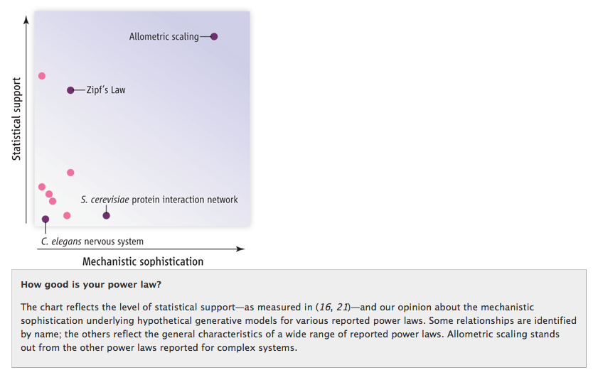
Anyway, the Science article is nice — it amusingly refers to certain statistical tests as “epically fail[ing]” — and it’s on the side of truth and goodness so it should be supported, BUT, it has one horrendous figure. I just love that, in this of all articles that should be harping on deeply flawed uses of (log-log) plots, they use one of those MBA-style bozo plots with unlabeled axes, one of which is viciously, unapologetically subjective:

If there is one power law I may single out for mercy in this delightful but verging-on-scary witch hunt, it would be Zipf’s law, cruelly put a bit low on that “mechanistic sophistication” axis. Zipf’s law has a wonderful explanation as the outcome of a Pitman-Yor process (going back to Simon 1955!), and Clauset/Shalizi/Newman found it was the only purported power law that actually checked out:

There is only one case—the distribution of the frequencies of occurrence of words
in English text—in which the power law appears to be truly convincing, in the sense
that it is an excellent fit to the data and none of the alternatives carries any weight.

Now, it is the case that the CRP/PYP/Yule-Simon stuff is still more of a statistical generative explanation than a deeper mechanistic one; but no one knows how cognition works, there are no satisfying causal stories for linguistic production, and it’s probably fundamentally unknowable anyways, so that’s the best science you can get. yay.

4 Comments

Histograms — matplotlib vs. R

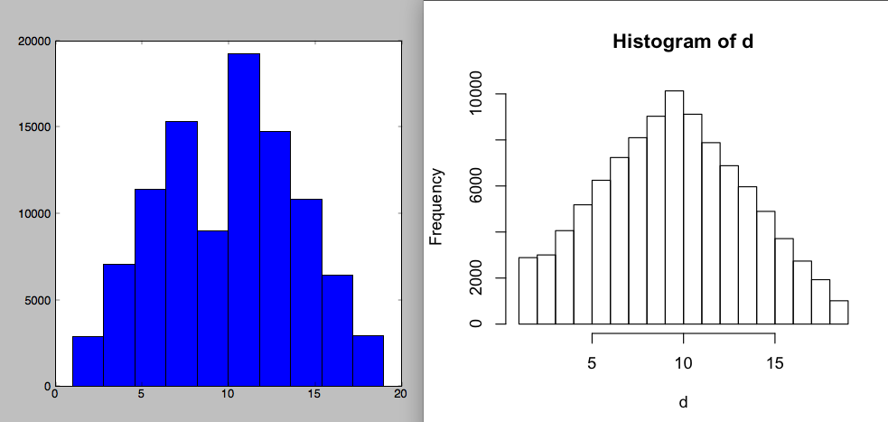
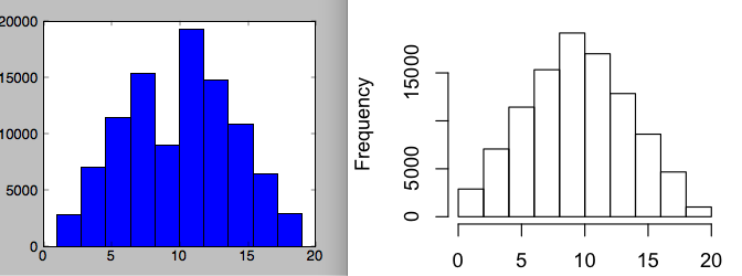
When possible, I like to use R for its really, really good statistical visualization capabilities. I’m doing a modeling project in Python right now (R is too slow, bad at large data, bad at structured data, etc.), and in comparison to base R, the matplotlib library is just painful. I wrote a toy Metropolis sampler for a triangle distribution and all I want to see is whether it looks like it’s working. For the same dataset, here are histograms with default settings. (Python: pylab.hist(d), R: hist(d))

I want to know whether my Metropolis sampler is working; those two plots give a very different idea. Of course, you could say this is an unfair comparison, since matplotlib is only using 10 bins, while R is using 18 here — and it’s always important to vary the bin size a few times when looking at histograms. But R’s defaults really are better: it actually uses an adaptive bin size, and the heuristic worked, choosing a reasonable number for the data. The hist() manual says it’s from Sturges (1926). It’s hard to find other computer software that cites 100 year old papers for its design decisions — and where it matters. (Old versions of R used to yell at you when you made a pie chart, citing perceptual studies that humans are really bad at interpreting them (here). This is what originally made me love R.)

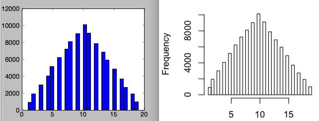
Second, R is much smarter about breakpoints. In the following plots, I’ve manually set the number of bins to 10, and then 30 for each.

The second one is now OK for matplotlib — it’s good enough to figure out what’s going on — though still a little lame. Why the gaps?

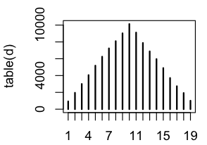
The problem is that my data are discrete — they’re all integers from 1 through 19 — and I think matplotlib is naively carving up that range into bins, which sometimes lumps together two integers, and sometimes gets zero of them. I understand this is the simple naive implementation, and you could say it’s my fault that I shouldn’t have used the pylab histogram function for this type of data — but it’s really not as good as whatever R is doing, which works rather well here, and I didn’t have to waste time thinking about the internals of the algorithm. For reference, here is the correct visualization of the data (R: plot(table(d))). Note that R’s original Sturges breakpoints did make one error: the first two values got combined into one bin.

Lessons: (1) always vary the bin sizes for histograms, especially if you’re using naive breakpoint selection, and (2) don’t ignore a century’s worth of statistical research on these issues. And since it’s hard to learn a century’s worth of statistics, just use R, where they’re compiled it in for you.

8 Comments

Bayes update view of pointwise mutual information


This is fun. Pointwise Mutual Information (e.g. Church and Hanks 1990) between two variable outcomes \(x\) and \(y\) is

\[ PMI(x,y) = \log \frac{p(x,y)}{p(x)p(y)} \]

It’s called “pointwise” because Mutual Information, between two (discrete) variables X and Y, is the expectation of PMI over possible outcomes of X and Y: \( MI(X,Y) = \sum_{x,y} p(x,y) PMI(x,y) \).

One interpretation of PMI is it’s measuring how much deviation from independence there is — since \(p(x,y)=p(x)p(y)\) if X and Y were independent, so the ratio is how non-independent they (the outcomes) are.

You can get another interpretation of this quantity if you switch into conditional probabilities. Looking just at the ratio, apply the definition of conditional probability:

\[ \frac{p(x,y)}{p(x)p(y)} = \frac{p(x|y)}{p(x)} \]

Think about doing a Bayes update for your belief about \(x\). Start with the prior \(p(x)\), then learn \(y\) and you update to the posterior belief \(p(x|y)\). How much your belief changes is measured by that ratio; the log-scaled ratio is PMI. (Positive PMI = increase belief, negative PMI = decrease belief. Positive vs. negative associations.)

Interestingly, it’s symmetric (obvious from the original definition of PMI, sure):
\[ \frac{p(x|y)}{p(x)} = \frac{p(y|x)}{p(y)} \]

So under this measurement of “amount of information you learn,” the amount you learn about \(x\) from \(y\) is actually the same as how much you learn about \(y\) from \(x\).

This is closer to the information gain view of mutual information, when you decompose it into relative and conditional entropies; the current Wikipedia page has some of the derivations back and forth for them.

Lots more about this stuff on the MI and KL Divergence Wikipedia pages. And early chapters of the (free) MacKay 2003 textbook. There seems to be lots of recent work using PMI for association scores between words or concepts and such (I did this with Facebook “Like” data at my internship there, it is quite fun); it’s nice because with MLE or fixed-Dirichlet-MAP estimation it only requires simple counts and no optimization/sampling, so you can use it on very large datasets, and it seems to give good pairwise association results in many circumstances.

Leave a comment